# HIDDEN
# Clear previously defined variables
%reset -f

# Set directory for data loading to work properly
import os
os.chdir(os.path.expanduser('~/notebooks/17'))
# HIDDEN
import warnings
# Ignore numpy dtype warnings. These warnings are caused by an interaction
# between numpy and Cython and can be safely ignored.
# Reference: https://stackoverflow.com/a/40846742
warnings.filterwarnings("ignore", message="numpy.dtype size changed")
warnings.filterwarnings("ignore", message="numpy.ufunc size changed")

import numpy as np
import matplotlib.pyplot as plt
import pandas as pd
import seaborn as sns
%matplotlib inline
import ipywidgets as widgets
from ipywidgets import interact, interactive, fixed, interact_manual
import nbinteract as nbi

sns.set()
sns.set_context('talk')
np.set_printoptions(threshold=20, precision=2, suppress=True)
pd.options.display.max_rows = 7
pd.options.display.max_columns = 8
pd.set_option('precision', 2)
# This option stops scientific notation for pandas
# pd.set_option('display.float_format', '{:.2f}'.format)
# HIDDEN
def df_interact(df, nrows=7, ncols=7):
    '''
    Outputs sliders that show rows and columns of df
    '''
    def peek(row=0, col=0):
        return df.iloc[row:row + nrows, col:col + ncols]
    if len(df.columns) <= ncols:
        interact(peek, row=(0, len(df) - nrows, nrows), col=fixed(0))
    else:
        interact(peek,
                 row=(0, len(df) - nrows, nrows),
                 col=(0, len(df.columns) - ncols))
    print('({} rows, {} columns) total'.format(df.shape[0], df.shape[1]))
# HIDDEN
def jitter_df(df, x_col, y_col):
    x_jittered = df[x_col] + np.random.normal(scale=0, size=len(df))
    y_jittered = df[y_col] + np.random.normal(scale=0.05, size=len(df))
    return df.assign(**{x_col: x_jittered, y_col: y_jittered})
Regression on Probabilities
In basketball, players score by shooting a ball through a hoop. One such player, LeBron James, is widely considered one of the best basketball players ever for his incredible ability to score.

LeBron plays in the National Basketball Association (NBA), the United States's premier basketball league. We've collected a dataset of all of LeBron's attempts in the 2017 NBA Playoff Games using the NBA statistics website (https://stats.nba.com/).
lebron = pd.read_csv('lebron.csv')
lebron
Each row of this dataset contains the following attributes of a shot LeBron attempted:
game_date: The date of the game.minute: The minute that the shot was attempted (each NBA game is 48 minutes long).opponent: The team abbreviation of LeBron's opponent.action_type: The type of action leading up to the shot.shot_type': The type of shot (either a 2 point shot or 3 point shot).shot_distance: LeBron's distance from the basket when the shot was attempted (ft).shot_made:0if the shot missed,1if the shot went in.
We would like to use this dataset to predict whether LeBron will make future shots. This is a classification problem; we predict a category, not a continuous number as we do in regression.
We may reframe this classification problem as a type of regression problem by predicting the probability that a shot will go in. For example, we expect that the probability that LeBron makes a shot is lower when he is farther away from the basket.
We plot the shot attempts below, showing the distance from the basket on the x-axis and whether he made the shot on the y-axis. Jittering the points slightly on the y-axis mitigates overplotting.
# HIDDEN
np.random.seed(42)
sns.lmplot(x='shot_distance', y='shot_made',
           data=jitter_df(lebron, 'shot_distance', 'shot_made'),
           fit_reg=False,
           scatter_kws={'alpha': 0.3})
plt.title('LeBron Shot Make vs. Shot Distance');
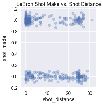
We can see that LeBron tends to make most shots when he is within five feet of the basket. A simple least squares linear regression model fit on this data produces the following predictions:
# HIDDEN
np.random.seed(42)
sns.lmplot(x='shot_distance', y='shot_made',
           data=jitter_df(lebron, 'shot_distance', 'shot_made'),
           ci=None,
           scatter_kws={'alpha': 0.4})
plt.title('Simple Linear Regression');
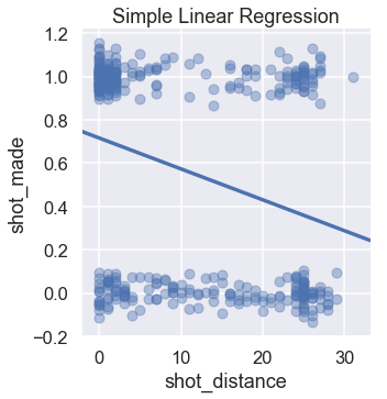
Linear regression predicts a continuous value. To perform classification, however, we need to convert this value into a category: a shot make or miss. We can accomplish this by setting a cutoff, or classification threshold. If the regression predicts a value greater than 0.5, we predict that the shot will make. Otherwise, we predict that the shot will miss.
We draw the cutoff below as a green dashed line. According to this cutoff, our model predicts that LeBron will make a shot if he is within 15 feet of the basket.
# HIDDEN
np.random.seed(42)
sns.lmplot(x='shot_distance', y='shot_made',
           data=jitter_df(lebron, 'shot_distance', 'shot_made'),
           ci=None,
           scatter_kws={'alpha': 0.4})
plt.axhline(y=0.5, linestyle='--', c='g')
plt.title('Cutoff for Classification');
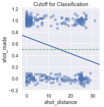
In the steps above, we attempt to perform a regression to predict the probability that a shot will go in. If our regression produces a probability, setting a cutoff of 0.5 means that we predict that a shot will go in when our model thinks the shot going in is more likely than the shot missing. We will revisit the topic of classification thresholds later in the chapter.
Issues with Linear Regression for Probabilities
Unfortunately, our linear model's predictions cannot be interpreted as probabilities. Valid probabilities must lie between zero and one, but our linear model violates this condition. For example, the probability that LeBron makes a shot when he is 100 feet away from the basket should be close to zero. In this case, however, our model will predict a negative value.
If we alter our regression model so that its predictions may be interpreted as probabilities, we will have no qualms about using its predictions for classification. We accomplish this with a new prediction function and a new loss function. The resulting model is called a logistic model.