# HIDDEN
# Clear previously defined variables
%reset -f

# Set directory for data loading to work properly
import os
os.chdir(os.path.expanduser('~/notebooks/11'))
# HIDDEN
import warnings
# Ignore numpy dtype warnings. These warnings are caused by an interaction
# between numpy and Cython and can be safely ignored.
# Reference: https://stackoverflow.com/a/40846742
warnings.filterwarnings("ignore", message="numpy.dtype size changed")
warnings.filterwarnings("ignore", message="numpy.ufunc size changed")

import numpy as np
import matplotlib.pyplot as plt
import pandas as pd
import seaborn as sns
%matplotlib inline
import ipywidgets as widgets
from ipywidgets import interact, interactive, fixed, interact_manual
import nbinteract as nbi

sns.set()
sns.set_context('talk')
np.set_printoptions(threshold=20, precision=2, suppress=True)
pd.options.display.max_rows = 7
pd.options.display.max_columns = 8
pd.set_option('precision', 2)
# This option stops scientific notation for pandas
# pd.set_option('display.float_format', '{:.2f}'.format)
# HIDDEN
def mse(theta, y_vals):
    return np.mean((y_vals - theta) ** 2)

def points_and_loss(y_vals, xlim, loss_fn):
    thetas = np.arange(xlim[0], xlim[1] + 0.01, 0.05)
    losses = [loss_fn(theta, y_vals) for theta in thetas]

    plt.figure(figsize=(9, 2))

    ax = plt.subplot(121)
    sns.rugplot(y_vals, height=0.3, ax=ax)
    plt.xlim(*xlim)
    plt.title('Points')
    plt.xlabel('Tip Percent')

    ax = plt.subplot(122)
    plt.plot(thetas, losses)
    plt.xlim(*xlim)
    plt.title(loss_fn.__name__)
    plt.xlabel(r'$ \theta $')
    plt.ylabel('Loss')
    plt.legend()
Loss Minimization Using a Program
Let us return to our constant model:
$$ \theta = C $$
We will use the mean squared error loss function:
$$ \begin{aligned} L(\theta, \textbf{y}) &= \frac{1}{n} \sum_{i = 1}^{n}(y_i - \theta)^2\\ \end{aligned} $$
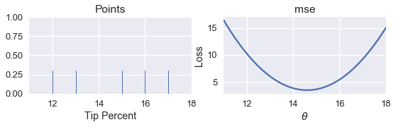
For simplicity, we will use the dataset $ \textbf{y} = [ 12, 13, 15, 16, 17 ] $. We know from our analytical approach in a previous chapter that the minimizing $ \theta $ for the MSE is $ \text{mean}(\textbf{y}) = 14.6 $. Let's see whether we can find the same value by writing a program.
If we write the program well, we will be able to use the same program on any loss function in order to find the minimizing value of $ \theta $, including the mathematically complicated Huber loss:
$$ L_\alpha(\theta, \textbf{y}) = \frac{1}{n} \sum_{i=1}^n \begin{cases} \frac{1}{2}(y_i - \theta)^2 & | y_i - \theta | \le \alpha \\ \alpha ( |y_i - \theta| - \frac{1}{2}\alpha ) & \text{otherwise} \end{cases} $$
First, we create a rug plot of the data points. To the right of the rug plot we plot the MSE for different values of $ \theta $.
# HIDDEN
pts = np.array([12, 13, 15, 16, 17])
points_and_loss(pts, (11, 18), mse)
How might we write a program to automatically find the minimizing value of $ \theta $? The simplest method is to compute the loss for many values $ \theta $. Then, we can return the $ \theta $ value that resulted in the least loss.
We define a function called simple_minimize that takes in a loss function, an array of data points, and an array of $\theta$ values to try.
def simple_minimize(loss_fn, dataset, thetas):
    '''
    Returns the value of theta in thetas that produces the least loss
    on a given dataset.
    '''
    losses = [loss_fn(theta, dataset) for theta in thetas]
    return thetas[np.argmin(losses)]
Then, we can define a function to compute the MSE and pass it into simple_minimize.
def mse(theta, dataset):
    return np.mean((dataset - theta) ** 2)

dataset = np.array([12, 13, 15, 16, 17])
thetas = np.arange(12, 18, 0.1)

simple_minimize(mse, dataset, thetas)
This is close to the expected value:
# Compute the minimizing theta using the analytical formula
np.mean(dataset)
Now, we can define a function to compute the Huber loss and plot the loss against $\theta $.
def huber_loss(theta, dataset, alpha = 1):
    d = np.abs(theta - dataset)
    return np.mean(
        np.where(d < alpha,
                 (theta - dataset)**2 / 2.0,
                 alpha * (d - alpha / 2.0))
    )
# HIDDEN
points_and_loss(pts, (11, 18), huber_loss)
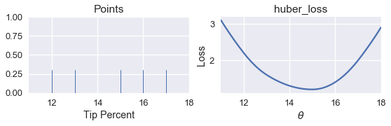
Although we can see that the minimizing value of $ \theta $ should be close to 15, we do not have an analytical method of finding $ \theta $ directly for the Huber loss. Instead, we can use our simple_minimize function.
simple_minimize(huber_loss, dataset, thetas)
Now, we can return to our original dataset of tip percentages and find the best value for $ \theta $ using the Huber loss.
tips = sns.load_dataset('tips')
tips['pcttip'] = tips['tip'] / tips['total_bill'] * 100
tips.head()
# HIDDEN
points_and_loss(tips['pcttip'], (11, 20), huber_loss)
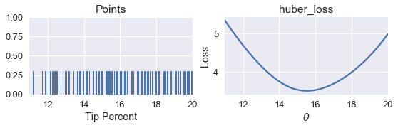
simple_minimize(huber_loss, tips['pcttip'], thetas)
We can see that using the Huber loss gives us $ \hat{\theta} = 15.5 $. We can now compare the minimizing $\hat{\theta} $ values for MSE, MAE, and Huber loss.
print(f"               MSE: theta_hat = {tips['pcttip'].mean():.2f}")
print(f"               MAE: theta_hat = {tips['pcttip'].median():.2f}")
print(f"        Huber loss: theta_hat = 15.50")
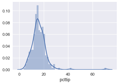
We can see that the Huber loss is closer to the MAE since it is less affected by the outliers on the right side of the tip percentage distribution:
sns.distplot(tips['pcttip'], bins=50);
Issues with simple_minimize
Although simple_minimize allows us to minimize loss functions, it has some flaws that make it unsuitable for general purpose use. Its primary issue is that it only works with predetermined values of $ \theta $ to test. For example, in this code snippet we used above, we had to manually define $ \theta $ values in between 12 and 18.
dataset = np.array([12, 13, 15, 16, 17])
thetas = np.arange(12, 18, 0.1)

simple_minimize(mse, dataset, thetas)
How did we know to examine the range between 12 and 18? We had to inspect the plot of the loss function manually and see that there was a minima in that range. This process becomes impractical as we add extra complexity to our models. In addition, we manually specified a step size of 0.1 in the code above. However, if the optimal value of $ \theta $ were 12.043, our simple_minimize function would round to 12.00, the nearest multiple of 0.1.
We can solve both of these issues at once by using a method called gradient descent.