L2 Regularization: Ridge Regression¶

In this section we introduce $ L_2 $ regularization, a method of penalizing large weights in our cost function to lower model variance. We briefly review linear regression, then introduce regularization as a modification to the cost function.

To perform least squares linear regression, we use the model:

$$ f_\hat{\theta}(x) = \hat{\theta} \cdot x $$

We fit the model by minimizing the mean squared error cost function:

$$ \begin{aligned} L(\hat{\theta}, X, y) &= \frac{1}{n} \sum_{i}^n(y_i - f_\hat{\theta} (X_i))^2\\ \end{aligned} $$

In the above definitions, $ X $ represents the $ n \times p $ data matrix, $ x $ represents a row of $ X $, $ y $ represents the observed outcomes, and $ \hat{\theta} $ represents the model weights.

L2 Regularization Definition¶

To add $ L_2 $ regularization to the model, we modify the cost function above:

$$ \begin{aligned} L(\hat{\theta}, X, y) &= \frac{1}{n} \sum_{i}(yi - f\hat{\theta} (X_i))^2

+ \lambda \sum_{j = 1}^{p} \hat{\theta_j}^2

\end{aligned} $$

Notice that the cost function above is the same as before with the addition of the $ L_2 $ regularization $ \lambda \sum_{j = 1}^{p} \hat{\theta_j}^2 $ term. The summation in this term sums the square of each model weight $ \hat{\theta_1}, \hat{\theta_2}, \ldots, \hat{\theta_p} $. The term also introduces a new scalar model parameter $ \lambda $ that adjusts the regularization penalty.

The regularization term causes the cost to increase if the values in $ \hat{\theta} $ are further away from 0. With the addition of regularization, the optimal model weights minimize the combination of loss and regularization penalty rather than the loss alone. Since the resulting model weights tend to be smaller in absolute value, the model has lower variance and higher bias.

Using $ L_2 $ regularization with a linear model and the mean squared error cost function is also known more commonly as ridge regression.

The Regularization Parameter¶

The regularization parameter $ \lambda $ controls the regularization penalty. A small $ \lambda $ results in a small penalty—if $ \lambda = 0 $ the regularization term is also $ 0 $ and the cost is not regularized at all.

A large $ \lambda $ terms results in a large penalty and therefore a simpler model. Increasing $ \lambda $ decreases the variance and increases the bias of the model. We use cross-validation to select the value of $ \lambda $ that minimizes the validation error.

Note about regularization in scikit-learn:

scikit-learn provides regression models that have regularization built-in. For example, to conduct ridge regression you may use the sklearn.linear_model.Ridge regression model. Note that scikit-learn models call the regularization parameter alpha instead of $ \lambda $.

scikit-learn conveniently provides regularized models that perform cross-validation to select a good value of $ \lambda $. For example, the sklearn.linear_model.RidgeCV allows users to input regularization parameter values and will automatically use cross-validation to select the parameter value with the least validation error.

Bias Term Exclusion¶

Note that the bias term $ \theta_0 $ is not included in the summation of the regularization term. We do not penalize the bias term because increasing the bias term does not increase the variance of our model—the bias term simply shifts all predictions by a constant value.

Data Normalization¶

Notice that the regularization term $ \lambda \sum_{j = 1}^{p} \hat{\theta_j}^2 $ penalizes each $ \hat{\theta_j} $ equally. However, the effect of each $ \hat{\theta_j} $ differs depending on the data itself. Consider this section of the water flow dataset after adding degree 8 polynomial features:

We can see that the degree 7 polynomial features have much larger values than the degree 1 features. This means that a large model weight for the degree 7 features affects the predictions much more than a large model weight for the degree 1 features. If we apply regularization to this data directly, the regularization penalty will disproportionately lower the model weight for the lower degree features. In practice, this often results in high model variance even after applying regularization since the features with large effect on prediction will not be affected.

To combat this, we normalize each data column by subtracting the mean and scaling the values in each column to be between -1 and 1. In scikit-learn, most regression models allow initializing with normalize=True to normalize the data before fitting.

Another analogous technique is standardizing the data columns by subtracting the mean and dividing by the standard deviation for each data column.

Using Ridge Regression¶

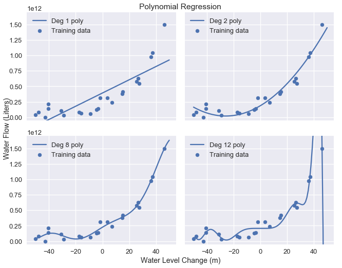
We have previously used polynomial features to fit polynomials of degree 2, 8, and 12 to water flow data. The original data and resulting model predictions are repeated below.

To conduct ridge regression, we first extract the data matrix and the vector of outcomes from the data:

Then, we apply a degree 12 polynomial transform to X:

We specify alpha values that scikit-learn will select from using cross-validation, then use the RidgeCV classifier to fit the transformed data.

Finally, we plot the model predictions for the base degree 8 polynomial classifier next to the regularized degree 8 classifier:

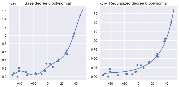
We can see that the regularized polynomial is smoother than the base degree 8 polynomial and still captures the major trend in the data.

Comparing the coefficients of the non-regularized and regularized models shows that ridge regression favors placing model weights on the lower degree polynomial terms:

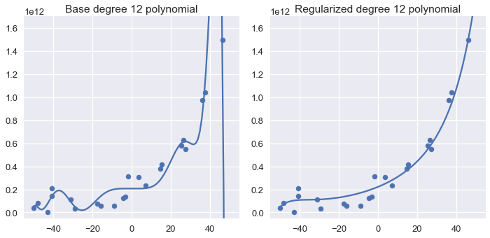
Repeating the process for degree 12 polynomial features results in a similar result:

Increasing the regularization parameter results in progressively simpler models. The plot below demonstrates the effects of increasing the regularization amount from 0.001 to 100.0.

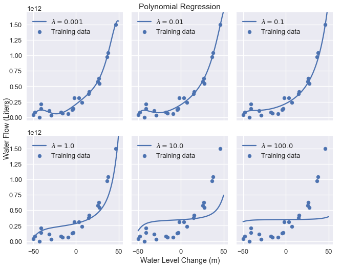
As we can see, increasing the regularization parameter increases the bias of our model. If our parameter is too large, the model becomes a constant model because any non-zero model weight is heavily penalized.

Summary¶

Using $ L_2 $ regularization allows us to tune model bias and variance by penalizing large model weights. $ L_2 $ regularization for least squares linear regression is also known by the more common name ridge regression. Using regularization adds an additional model parameter $ \lambda $ that we adjust using cross-validation.