# HIDDEN
# Clear previously defined variables
%reset -f

# Set directory for data loading to work properly
import os
os.chdir(os.path.expanduser('~/notebooks/17'))
# HIDDEN
import warnings
# Ignore numpy dtype warnings. These warnings are caused by an interaction
# between numpy and Cython and can be safely ignored.
# Reference: https://stackoverflow.com/a/40846742
warnings.filterwarnings("ignore", message="numpy.dtype size changed")
warnings.filterwarnings("ignore", message="numpy.ufunc size changed")

import numpy as np
import matplotlib.pyplot as plt
import pandas as pd
import seaborn as sns
%matplotlib inline
import ipywidgets as widgets
from ipywidgets import interact, interactive, fixed, interact_manual
import nbinteract as nbi

sns.set()
sns.set_context('talk')
np.set_printoptions(threshold=20, precision=2, suppress=True)
pd.options.display.max_rows = 7
pd.options.display.max_columns = 8
pd.set_option('precision', 2)
# This option stops scientific notation for pandas
# pd.set_option('display.float_format', '{:.2f}'.format)
# HIDDEN
def df_interact(df, nrows=7, ncols=7):
    '''
    Outputs sliders that show rows and columns of df
    '''
    def peek(row=0, col=0):
        return df.iloc[row:row + nrows, col:col + ncols]
    if len(df.columns) <= ncols:
        interact(peek, row=(0, len(df) - nrows, nrows), col=fixed(0))
    else:
        interact(peek,
                 row=(0, len(df) - nrows, nrows),
                 col=(0, len(df.columns) - ncols))
    print('({} rows, {} columns) total'.format(df.shape[0], df.shape[1]))
# HIDDEN
from scipy.optimize import minimize as sci_min
def minimize(cost_fn, grad_cost_fn, X, y, progress=True):
    '''
    Uses scipy.minimize to minimize cost_fn using a form of gradient descent.
    '''
    theta = np.zeros(X.shape[1])
    iters = 0

    def objective(theta):
        return cost_fn(theta, X, y)
    def gradient(theta):
        return grad_cost_fn(theta, X, y)
    def print_theta(theta):
        nonlocal iters
        if progress and iters % progress == 0:
            print(f'theta: {theta} | cost: {cost_fn(theta, X, y):.2f}')
        iters += 1

    print_theta(theta)
    return sci_min(
        objective, theta, method='BFGS', jac=gradient, callback=print_theta,
        tol=1e-7
    ).x
Using Logistic Regression
We have developed all the components of logistic regression. First, the logistic model used to predict probabilities:
$$ \begin{aligned} f_\hat{\boldsymbol{\theta}} (\textbf{x}) = \sigma(\hat{\boldsymbol{\theta}} \cdot \textbf{x}) \end{aligned} $$
Then, the cross-entropy loss function:
$$ \begin{aligned} L(\boldsymbol{\theta}, \textbf{X}, \textbf{y}) = &= \frac{1}{n} \sum_i \left(- y_i \ln \sigma_i - (1 - y_i) \ln (1 - \sigma_i ) \right) \\ \end{aligned} $$
Finally, the gradient of the cross-entropy loss for gradient descent:
$$ \begin{aligned} \nabla_{\boldsymbol{\theta}} L(\boldsymbol{\theta}, \textbf{X}, \textbf{y}) &= - \frac{1}{n} \sum_i \left( y_i - \sigma_i \right) \textbf{X}_i \\ \end{aligned} $$
In the expressions above, we let $ \textbf{X} $ represent the $ n \times p $ input data matrix, $\textbf{x}$ a row of $ \textbf{X} $, $ \textbf{y} $ the vector of observed data values, and $ f_\hat{\boldsymbol{\theta}}(\textbf{x}) $ the logistic model with optimal parameters $\hat{\boldsymbol{\theta}}$ . As a shorthand, we define $ \sigma_i = f_\hat{\boldsymbol{\theta}}(\textbf{X}_i) = \sigma(\textbf{X}_i \cdot \hat{\boldsymbol{\theta}}) $.
Logistic Regression on LeBron's Shots
Let us now return to the problem we faced at the start of this chapter: predicting which shots LeBron James will make. We start by loading the dataset of shots taken by LeBron in the 2017 NBA Playoffs.
lebron = pd.read_csv('lebron.csv')
lebron
We've included a widget below to allow you to pan through the entire DataFrame.
df_interact(lebron)
We start by using only the shot distance to predict whether or not the shot is made. scikit-learn conveniently provides a logistic regression classifier as the sklearn.linear_model.LogisticRegression class. To use the class, we first create our data matrix X and vector of observed outcomes y.
X = lebron[['shot_distance']].as_matrix()
y = lebron['shot_made'].as_matrix()
print('X:')
print(X)
print()
print('y:')
print(y)
As is customary, we split our data into a training set and a test set.
from sklearn.model_selection import train_test_split

X_train, X_test, y_train, y_test = train_test_split(
    X, y, test_size=40, random_state=42
)
print(f'Training set size: {len(y_train)}')
print(f'Test set size: {len(y_test)}')
scikit-learn makes it simple to initialize the classifier and fit it on X_train and y_train:
from sklearn.linear_model import LogisticRegression
simple_clf = LogisticRegression()
simple_clf.fit(X_train, y_train)
To visualize the classifier's performance, we plot the original points and the classifier's predicted probabilities.
# HIDDEN
np.random.seed(42)
sns.lmplot(x='shot_distance', y='shot_made',
           data=lebron,
           fit_reg=False, ci=False,
           y_jitter=0.1,
           scatter_kws={'alpha': 0.3})

xs = np.linspace(-2, 32, 100)
ys = simple_clf.predict_proba(xs.reshape(-1, 1))[:, 1]
plt.plot(xs, ys)

plt.title('LeBron Training Data and Predictions')
plt.xlabel('Distance from Basket (ft)')
plt.ylabel('Shot Made');
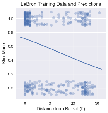
Evaluating the Classifier
One method to evaluate the effectiveness of our classifier is to check its prediction accuracy: what proportion of points does it predict correctly?
simple_clf.score(X_test, y_test)
Our classifier achieves a rather low accuracy of 0.60 on the test set. If our classifier simply guessed each point at random, we would expect an accuracy of 0.50. In fact, if our classifier simply predicted that every shot LeBron takes will go in, we would also get an accuracy of 0.60:
# Calculates the accuracy if we always predict 1
np.count_nonzero(y_test == 1) / len(y_test)
For this classifier, we only used one out of several possible features. As in multivariable linear regression, we will likely achieve a more accurate classifier by incorporating more features.
Multivariable Logistic Regression
Incorporating more numerical features in our classifier is as simple as extracting additional columns from the lebron DataFrame into the X matrix. Incorporating categorical features, on the other hand, requires us to apply a one-hot encoding. In the code below, we augment our classifier with the minute, opponent, action_type, and shot_type features, using the DictVectorizer class from scikit-learn to apply a one-hot encoding to the categorical variables.
from sklearn.feature_extraction import DictVectorizer

columns = ['shot_distance', 'minute', 'action_type', 'shot_type', 'opponent']
rows = lebron[columns].to_dict(orient='row')

onehot = DictVectorizer(sparse=False).fit(rows)
X = onehot.transform(rows)
y = lebron['shot_made'].as_matrix()

X.shape
We will again split the data into a training set and test set:
X_train, X_test, y_train, y_test = train_test_split(
    X, y, test_size=40, random_state=42
)
print(f'Training set size: {len(y_train)}')
print(f'Test set size: {len(y_test)}')
Finally, we fit our model once more and check its accuracy:
clf = LogisticRegression()
clf.fit(X_train, y_train)
print(f'Test set accuracy: {clf.score(X_test, y_test)}')
This classifier is around 12% more accurate than the classifier that only took the shot distance into account. In Section 17.7, we explore additional metrics used to evaluate classifier performance.
Summary
We have developed the mathematical and computational machinery needed to use logistic regression for classification. Logistic regression is widely used for its simplicity and effectiveness in prediction.