Fitting a Linear Model Using Gradient Descent¶

We want to fit a linear model that predicts the tip amount based on the total bill of the table:

$$ f_\boldsymbol\theta (x) = \theta_1 x + \theta_0 $$

In order to optimize $ \theta_1 $ and $ \theta_0 $, we need to first choose a loss function. We will choose the mean squared error loss function:

$$ \begin{aligned} L(\boldsymbol\theta, \textbf{x}, \textbf{y}) &= \frac{1}{n} \sum_{i = 1}^{n}(y_i - f_\boldsymbol\theta (x_i))^2\\ \end{aligned} $$

Note that we have modified our loss function to reflect the addition of an explanatory variable in our new model. Now, $ \textbf{x} $ is a vector containing the individual total bills, $ \textbf{y} $ is a vector containing the individual tip amounts, and $ \boldsymbol\theta $ is a vector: $ \boldsymbol\theta = [ \theta_1, \theta_0 ] $.

Using a linear model with the squared error also goes by the name of least-squares linear regression. We can use gradient descent to find the $ \boldsymbol\theta $ that minimizes the loss.

An Aside on Using Correlation

If you have seen least-squares linear regression before, you may recognize that we can compute the correlation coefficient and use it to determine $ \theta_1 $ and $ \theta_0 $. This is simpler and faster to compute than using gradient descent for this specific problem, similar to how computing the mean was simpler than using gradient descent to fit a constant model. We will use gradient descent anyway because it is a general-purpose method of loss minimization that still works when we later introduce models that do not have analytic solutions. In fact, in many real-world scenarios, we will use gradient descent even when an analytic solution exists because computing the analytic solution can take longer than gradient descent, especially on large datasets.

Derivative of the MSE Loss¶

In order to use gradient descent, we have to compute the derivative of the MSE loss with respect to $ \boldsymbol\theta $. Now that $ \boldsymbol\theta $ is a vector of length 2 instead of a scalar, $ \nabla_{\boldsymbol\theta} L(\boldsymbol\theta, \textbf{x}, \textbf{y}) $ will also be a vector of length 2.

$$ \begin{aligned} \nabla_{\boldsymbol\theta} L(\boldsymbol\theta, \textbf{x}, \textbf{y}) &= \nabla_{\boldsymbol\theta} \left[ \frac{1}{n} \sum_{i = 1}^{n}(y_i - f_\boldsymbol\theta (x_i))^2 \right] \\ &= \frac{1}{n} \sum_{i = 1}^{n}2 (y_i - f_\boldsymbol\theta (x_i))(- \nabla_{\boldsymbol\theta} f_\boldsymbol\theta (x_i))\\ &= -\frac{2}{n} \sum_{i = 1}^{n}(y_i - f_\boldsymbol\theta (x_i))(\nabla_{\boldsymbol\theta} f_\boldsymbol\theta (x_i))\\ \end{aligned} $$

We know:

$$ f_\boldsymbol\theta (x) = \theta_1 x + \theta_0 $$

We now need to compute $ \nabla_{\boldsymbol\theta} f_\boldsymbol\theta (x_i) $ which is a length 2 vector.

$$ \begin{aligned} \nabla_{\boldsymbol\theta} f_\boldsymbol\theta (x_i) &= \begin{bmatrix} \frac{\partial}{\partial \theta_0} f_\boldsymbol\theta (x_i)\\ \frac{\partial}{\partial \theta_1} f_\boldsymbol\theta (x_i) \end{bmatrix} \\ &= \begin{bmatrix} \frac{\partial}{\partial \theta_0} [\theta_1 x_i + \theta_0]\\ \frac{\partial}{\partial \theta_1} [\theta_1 x_i + \theta_0] \end{bmatrix} \\ &= \begin{bmatrix} 1 \\ x_i \end{bmatrix} \\ \end{aligned} $$

Finally, we plug back into our formula above to get

$$ \begin{aligned} \nabla_{\boldsymbol\theta} L(\theta, \textbf{x}, \textbf{y}) &= -\frac{2}{n} \sum_{i = 1}^{n}(y_i - f_\boldsymbol\theta (x_i))(\nabla_{\boldsymbol\theta} f_\boldsymbol\theta (x_i))\\ &= -\frac{2}{n} \sum_{i = 1}^{n} (y_i - f_\boldsymbol\theta (x_i)) \begin{bmatrix} 1 \\ x_i \end{bmatrix} \\ &= -\frac{2}{n} \sum_{i = 1}^{n} \begin{bmatrix} (y_i - f_\boldsymbol\theta (x_i)) \\ (y_i - f_\boldsymbol\theta (x_i)) x_i \end{bmatrix} \\ \end{aligned} $$

This is a length 2 vector since $ (y_i - f_\boldsymbol\theta (x_i)) $ is scalar.

Running Gradient Descent¶

Now, let's fit a linear model on the tips dataset to predict the tip amount from the total table bill.

First, we define a Python function to compute the loss:

Then, we define a function to compute the gradient of the loss:

We'll use the previously defined minimize function that runs gradient descent, accounting for our new explanatory variable. It has the function signature (body omitted):

minimize(loss_fn, grad_loss_fn, x_vals, y_vals)

Finally, we run gradient descent!

We can see that gradient descent converges to the theta values of $\hat\theta_0 = 0.01$ and $\hat\theta_1 = 0.14$. Our linear model is:

$$y = 0.14x + 0.01$$

We can use our estimated thetas to make and plot our predictions alongside the original data points.

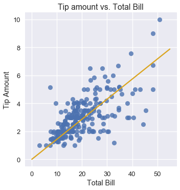
We can see that if a table's bill is $\$10$, our model will predict that the waiter gets around $\$1.50$ in tip. Similarly, if a table's bill is $\$40$, our model will predict a tip of around $\$6.00$.