GPU-Accelerated Symplectic Integrator — Mathematical Documentation

Overview

This document explains the mathematical foundations and numerical methods implemented in this project, with a focus on:

• Hamiltonian dynamics
• The Hénon–Heiles system
• Structure-preserving (symplectic) integration
• GPU-parallel execution

The goal is to simulate nonlinear dynamical systems faithfully over long time horizons, where naive high-accuracy methods often fail.

---

1. Hamiltonian Mechanics

1.1 Phase Space

The system evolves in a 4-dimensional phase space:

[ (q, p) = (x, y, p_x, p_y) ]

• (q = (x, y)): position
• (p = (p_x, p_y)): momentum

Phase Space Trajectory

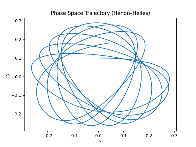
This shows the trajectory in configuration space ((x, y)). For chaotic regimes, the trajectory explores complex regions of phase space.

---

1.2 Hamiltonian Function

The total energy of the system is:

[ H(x,y,p_x,p_y) = T(p) + V(x,y) ]

with:

• Kinetic energy: [ T = \frac{1}{2}(p_x^2 + p_y^2) ]

• Potential energy (Hénon–Heiles): [ V(x,y) = \frac{1}{2}(x^2 + y^2) + x^2 y - \frac{1}{3} y^3 ]

---

1.3 Equations of Motion

Hamilton’s equations:

[ \dot{x} = p_x, \quad \dot{y} = p_y ] [ \dot{p}_x = -\frac{\partial V}{\partial x}, \quad \dot{p}_y = -\frac{\partial V}{\partial y} ]

---

1.4 Gradient of the Potential

[ \frac{\partial V}{\partial x} = x + 2xy ] [ \frac{\partial V}{\partial y} = y + x^2 - y^2 ]

These are computed in the CUDA device function:

compute_gradients(x, y, grad_x, grad_y)

---

2. Geometry of Hamiltonian Systems

Hamiltonian systems have special structure:

2.1 Phase Space Flow

        p
        ↑
        │        trajectories follow level sets of H
        │     ⟲      ⟲       ⟲
        │   ⟲    ⟲       ⟲
        │ ⟲
        └──────────────→ q

• Motion stays on constant-energy surfaces
• Flow is volume-preserving (Liouville’s theorem)

---

2.2 Key Invariants

• Energy (H) is conserved
• Phase-space volume is conserved
• Trajectories lie on manifolds

---

3. Numerical Integration Challenge

Standard methods (e.g., RK4):

• Minimize local truncation error
• Destroy global structure

Result:

Energy Conservation

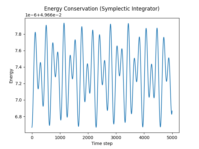
The symplectic integrator preserves energy up to bounded oscillations, demonstrating long-term stability.

---

4. Symplectic Integrator (Leapfrog / Verlet)

4.1 Algorithm

The symplectic method splits updates into half-step momentum and full-step position:

[ p_{n+1/2} = p_n - \frac{\Delta t}{2} \nabla V(q_n) ]

[ q_{n+1} = q_n + \Delta t , p_{n+1/2} ]

[ p_{n+1} = p_{n+1/2} - \frac{\Delta t}{2} \nabla V(q_{n+1}) ]

---

4.2 Geometric Interpretation

Instead of approximating the trajectory directly, we approximate the flow map:

Step splitting:

[Kick] → [Drift] → [Kick]

p ----> p_half ----> p_next
   \        |
    \       |
     \      v
       q --------> q_next

---

4.3 Why It Works

Symplectic integrators preserve:

• Phase-space structure
• Symplectic 2-form
• Long-term qualitative behavior

---

4.4 Energy Behavior

Instead of drifting:

Energy vs Time (Symplectic)

E
│   ~~~~~~~~
│  ~        ~
│ ~          ~
│~            ~
└────────────── t

Energy error is:

[ H(t) = H(0) + \mathcal{O}(\Delta t^2) ]

but remains bounded.

---

5. Comparison of Integrators

Method	Order	Symplectic	Energy Behavior	Long-Term Stability
Euler	1	❌	Diverges	❌
RK4	4	❌	Drifts slowly	❌
Leapfrog	2	✅	Oscillatory, bounded	✅

---

6. CUDA Parallelization Model

6.1 Problem Structure

Each trajectory evolves independently:

[ z_i(t) \rightarrow z_i(t + \Delta t) ]

---

6.2 GPU Mapping

Thread i  →  trajectory i

(x[i], y[i], px[i], py[i])

---

6.3 Memory Layout

Structure of Arrays (SoA):

x:   [x0 x1 x2 x3 ...]
y:   [y0 y1 y2 y3 ...]
px:  [p0 p1 p2 p3 ...]
py:  [p0 p1 p2 p3 ...]

Benefits:

• Coalesced memory access
• High bandwidth utilization

---

6.4 Kernel Execution

integrator_kernel<<<grid, block>>>(...)

Each thread performs:

for step in time:
    symplectic_update()

---

7. Energy Diagnostics

Energy is computed as:

[ E_i = \frac{1}{2}(p_x^2 + p_y^2) + V(x,y) ]

Used for:

• Verifying correctness
• Comparing integrators
• Detecting numerical instability

---

8. Key Insight

High-order accuracy is not enough for physical simulation.

• RK4: accurate trajectory locally, wrong globally
• Symplectic: slightly less accurate locally, correct physics globally

---

9. Extensions

9.1 Higher-Order Symplectic Methods

• Yoshida integrators
• Forest–Ruth splitting

---

9.2 Advanced Analysis

• Poincaré sections
• Lyapunov exponents
• Chaos detection

---

9.3 HPC Extensions

• Mixed precision (FP32/FP64 hybrid)
• Multi-GPU scaling
• Adaptive batching

---

10. Summary

This project demonstrates:

• How Hamiltonian structure drives algorithm choice
• Why symplectic integrators are essential
• How GPUs enable massively parallel trajectory simulation

---

11. Minimal Conceptual Diagram

Hamiltonian System
        ↓
Equations of Motion
        ↓
Discretization Choice
        ↓
 ┌───────────────┬─────────────────┐
 │ Standard ODE  │ Symplectic      │
 │ Methods       │ Integrators     │
 ├───────────────┼─────────────────┤
 │ RK4           │ Leapfrog        │
 │ High accuracy │ Structure-pres. │
 │ Energy drift  │ Energy bounded  │
 └───────────────┴─────────────────┘
        ↓
GPU Parallel Execution
        ↓
Millions of trajectories

---

Final Remark

This codebase is a compact example of a deep principle:

Preserving mathematical structure is often more important than minimizing numerical error.

This is especially true in:

• Computational physics
• Molecular dynamics
• Celestial mechanics
• Long-term dynamical simulations

---